Stellar feedback is an important aspect of galaxy formation. If you want to catch up, check out my other post on the the topic. One thing in particular that is important is how strong the stellar feedback is. If it's too weak, it won't do anything and all the gas will turn into stars; too strong and it will blow up the galaxy, ejecting the gas into the furthest reaches of space. It's a bit of a Goldilocks situation where stellar feedback has to have just the right amount of oomph to it in order to successfully regulate star formation in galaxies.

One way the strength of stellar feedback can change is how clustered in time and space supernovae occur. If you have ten supernovae going off all at the same time there's an outsized scaling effect that results in more than 10x the amount of energy of a single supernova going off. In this post, I'll describe a statistical model I developed to help understand how supernova clustering occurs in realistic simulations of a galaxy.

Developing a statistical model

To understand how supernovae are clustered in our realistic simualation, I compared the results of the simulation to simple parameterized pseudo-random model. The model was designed to measure the clustering statistics relevant to the strength of supernova feedback. Specifically, I wanted to understand how many supernovae were being launched within eachother's cooling radius (how big the blast wave gets before it cools down and mixes with the surrounding gas) within a cooling time (the amount of time it takes for the blastwave to get that big). More broadly, I wanted to understand how supernovae in our simulation are correlated both spatially and temporally.

I first defined the "clustering strength" as the size of a "cluster" of supernovae and the number of clusters of that size. I then developed a fancy recursive friends-of-friends algorithm to go out and measure the clustering strength in our simulation. The algorithm uses two dynamic linking lengths: one for the proximity in space and one for their proximity in time.

• proximity in space: I calculated the distance between two supernovae using their spatial coordinates (x, y, and z). I then compared it to the cooling radius of each supernova's hot bubble. The cooling radius can be thought of as the radius of influence around a supernova, within which it can potentially interact with other supernovae.

• proximity in time: Next, I compared each supernova's launch and cooling times. The idea was to ensures that a supernova can only be considered a "friend" of another if it is launched after the other supernova but before it cools down.

The friends-of-friends code iterates through all possible pairs of supernovae and checks these conditions to construct clusters of supernovae. It identifies friends, friends of friends, and so on until no more supernovae meet the criteria for cluster membership. Once a cluster is finished, the algorithm moves on to the next unprocessed supernova and starts building another cluster, continuing the process until all the supernovae have been evaluated.

Using this algorithm, I was able to take measurements of the simulation and determine what the "real" clustering strength was. The next step was to use a simple model to try and parameterize it.

Parameterizing the clustering strength with a broken power-law

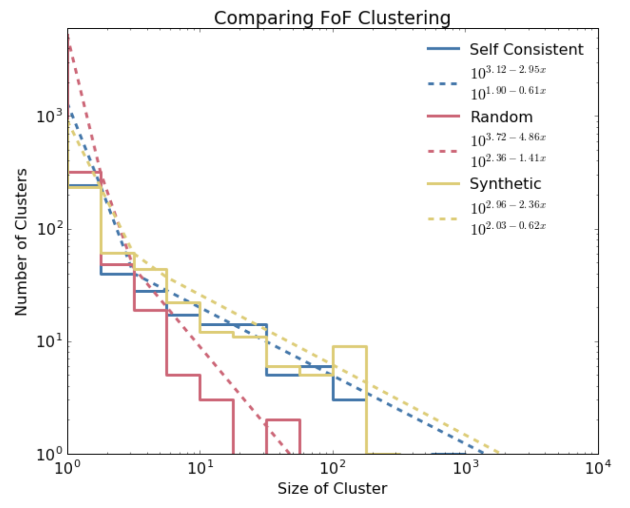
The output of my friends-of-friends code with supernovae taken from the simulation was a bunch of clusters of different sizes. Using that population of clusters I could pretty easily calculate the clustering strength by just taking a histogram of cluster sizes. When I did that, I noticed the histogram had a kind of distinctive shape: when plotted on a log-log axis it was kind of like a straight line-- but really it was like two with a joint in the middle between them. To test whether this shape was particular to the simulation I re-ran my friends-of-friends code but with input taken from just randomly assigned positions and launch times. By comparing the two, I could tell how much more correlated the supernovae in the simulation were compared to a random sample.

What I found was that while the parameters were different, both distributions could be pretty well described by a broken power law (check out the following graph). Using the form of a broken power law, I could then describe a probability distribution function and, crucially, sample it! Once I had the probability distribution function of the supernovae from the simulation I then wanted to see if it would be possible to replicate their statistics without having to re-run the simulation (which was very computationally expensive; millions of CPU hours and weeks of wall-time on our supercomputer).

Comparing the clustering strength of three different kinds of supernova seeding schemes: 1. what is done in the simulation (blue); 2. totally random (red); and 3. a modified pseudo-random method that seeks to imitate the simulation (yellow).

Applying the model to generate synthetic clusters more cheaply

To create synthetic clusters, I followed a simple prescription for generating randomly placed ad hoc clusters

1. I only "launched" as many supernovae as were observed in the simulation, and I distributed the launch times uniformly
2. I randomly picked a cluster size according to the parameterized probability distribution of the clustering strength
3. I placed the first member randomly in a rectangular slab representing the area where the bulk of the galactic disk is (that's the square edges in the image at the top of this page).
4. I iteratively added subsequent members by randomly selecting an unassigned supernova and a random member of the cluster. I then placed the unassigned supernova at a random location within the cluster member's cooling radius (ensuring it would be identified as part of the cluster in my friends-of-friends code).
5. I continued until I ran out of unassigned supernovae

This approach to generating synthetic supernova clusters is highly adaptable to any arbitrary PDF, allowing for all sorts of flexibility. To test my methodology I re-ran my friends-of-friends code on the synthetic population of supernovae and indeed was able to extract the clustering strength I had hoped to emulate. However, very interestingly, the global geometry was way different! If you look at the image at the top of the page, you'll see that the yellow dots are distributed pretty evenly throughout the disk whereas the blue dots follow a distinctive spiral pattern.

Closing thoughts and the relevance to data science and software engineering more broadly

In conclusion, my methodology demonstrated the potential of data science and software engineering to answer "real-life" questions. By articulating our question in terms of a statistical concept (friends-of-friends clusters) and applying the necessary software engineering skills to build the necessary framework (including multithreading and accounting for memory limitations using e.g. a sliding memory buffer) I was able to develop a statistical model and gain a better understanding of the underlying processes that govern the behavior of galaxies. Still, while this approach shows promise, there is still room for improvement in order to fully capture the details of the clustering statistics in simulations-- in particular the spiral geometry.

If you want to know more you can check out the writeup that I put together.